One workspace. A growing scientific investigation.
Follow climate experiments, fluid dynamics, and geophysical inference alongside the setup and analysis needed to carry out the work.
A scientific project develops through questions, runs, and revisions. Here, requests, outputs, and open questions remain connected as the investigation expands across different physical systems.
10 recorded sessions: 6 scientific studies, 3 engineering notes, and 1 unresolved CFD investigation. These are demonstrations of computational work, not measured customer outcomes.
Model inputs + numerical outputs + explanations + next experiments
Editorial grouping of related capabilities, not a proven serial dependency graph. Sessions overlap; the exports do not establish that every later study reused an unchanged earlier specialist.
How Laplace carried the project work
Direct the investigation. Inspect the work.
Laplace carries technical execution while researchers set the question, steer the study, and evaluate the evidence.
A team-managed workflowIllustrative workflow with existing tools
Task 1Assemble environments
→
Task 2Learn each solver
→
Task 3Configure + run
→
Task 4Reconcile outputs
→
Task 5Prepare explanations
The team coordinates tools, context, and revisions across the study.
With LaplaceTechnical work demonstrated in these studies
Six controlled experiments distinguish the change in energy balance from the temperature response.
Idealized aquaplanet with a 30 m slab ocean, without realistic land, sea ice, seasons, or ocean circulation. These responses are not an Earth climate-sensitivity estimate.
Run a minimal CESM infrastructure test: compset X with dead model components, resolution f19_g17, and a one-day run. Create the case, build it, submit it, confirm time-stepping and summarize the output.Run a minimal CESM infrastructure test: compset X with dead model components, resolution f19_g17, and a one-day run. Create the case, build it, submit it, confirm time-stepping and summarize the output.Run a minimal CESM infrastructure test: compset X with dead model components, resolution f19_g17, and a one-day run. Create the case, build it, submit it, confirm time-stepping and summarize the output.
Research prompt↑
LLaplaceRecorded result
A completed build-to-output check.
The record reports a one-model-day smoke test, a 35-second model execution, and restart output. This established an infrastructure receipt for subsequent work.
Infrastructure smoke test with dead model components. No climate finding is claimed.
The result summarizes the recorded session, including later requests and review.
Read the research prompt
Research prompt · edited for public presentation
Run a minimal CESM infrastructure test: compset X with dead model components, resolution f19_g17, and a one-day run. Create the case, build it, submit it, confirm time-stepping and summarize the output.
A minimal test checks compilation, submission, time-stepping and output recovery before a larger workload begins.
Build and execution are separate clocks from the supplied report. Dead model components test the infrastructure; this is not a climate result.
Prove the run path before committing to a larger study.
Think of this as testing a factory line before producing anything valuable. The output is confidence that the machinery can start, advance time and finish. It does not yet tell us anything about the climate.
Study scope. Infrastructure smoke test with dead model components. No climate finding is claimed.
A large scientific run is a poor place to discover that compilation, job submission or output collection is broken.
01
Specify a minimal acceptance test
The user explicitly requested dead model components and one model day, to prove the pipeline rather than perform science.
02
Build, submit and inspect
The supplied report records case creation, a 289-second build, cluster submission and 48 coupler steps of 1,800 seconds.
03
Leave a bounded infrastructure receipt
The report records a 35-second model execution and restart output. A claim that the case name automatically selected test mode was retracted.
How Laplace carried the work
Direct the investigation. Inspect the work.
Laplace carries technical execution while researchers set the question, steer the study, and evaluate the evidence.
A team-managed workflowIllustrative workflow with existing tools
Task 1Define acceptance
→
Task 2Configure CESM
→
Task 3Build + submit
→
Task 4Inspect logs
→
Task 5Record the result
The team coordinates tools, context, and revisions across the study.
With LaplaceTechnical work demonstrated in these studies
HUMANBrief + steer
Laplace carries the technical work
Build caseCompile + submitInspect + report
↺ Run → inspect → revise, with researcher steering
HUMANReview + decide
Setup work delegatedCase creation, build, submission and inspection are captured together.
An early failure gateThe minimal run checks infrastructure before a larger science workload.
Reusable acceptance recordThe report makes the successful path and its limits inspectable.
Illustrates work ownership. Box widths are schematic; human time saved was not measured.
Inspect the work inside the Laplace block
Build case. The user explicitly requested dead model components and one model day, to prove the pipeline rather than perform science.
Compile + submit. The supplied report records case creation, a 289-second build, cluster submission and 48 coupler steps of 1,800 seconds.
Inspect + report. The report records a 35-second model execution and restart output. A claim that the case name automatically selected test mode was retracted.
These investigations often continued across separate visits. The first and last messages do not measure continuous work.
00h 39m 32sCalendar span of the conversation
3mCombined child-agent windows, with overlapping intervals counted once
Agent windows can include waiting and omit work in the main conversation. They are not a measure of active human work, total compute or time saved. The exports do not provide a reliable labour clock.
Scientific assumptions and limitations
This is an infrastructure smoke test with dead components, not a climate simulation.
The ZIP supplies a report, not the raw logs or a complete reconstruction package.
The report retracts the automatic run-type claim; registry upload was not completed.
The next useful decision
Advance to a real-physics configuration and verify its input data and output fields.
Run a small CESM real-physics smoke test, from case setup through completed output.Run a small CESM real-physics smoke test, from case setup through completed output.Run a small CESM real-physics smoke test, from case setup through completed output.
Research prompt↑
LLaplaceRecorded result
Ten days of growing weather patterns.
Expanded from the initial one-day request, the investigation produced a ten-day atmospheric-wave study, diagnostic tables, a globe artifact, and explanatory movies.
Idealized model dynamics. The 214× figure measures pressure-wave growth, not computational speed or forecast accuracy.
Playback length is separate from simulated time and the session span.
A small disturbance becomes ten days of explainable weather.
Uneven heating gives the atmosphere energy. An initially small disturbance can grow into large weather patterns. Here, the value is a connected path from a model setup to data, charts and a movie that explain that mechanism.
Study scope. Idealized model dynamics. The 214× figure measures pressure-wave growth, not computational speed or forecast accuracy.
214×Pressure-wave amplitude, day 1 → day 10; a physical growth ratioSource ↗
10 daysWindow covered by the selected lifecycle explanationSource ↗
Original corrected chart. Daily-mean cloud-water maxima remain below the plotted 1,000 mg/kg threshold.
How the investigation developed.
Getting a model to finish is only the first step. Someone still has to identify the mechanism, extract the right quantities and make the result understandable.
01
Run an idealized physical atmosphere
The initial request was a one-day FKESSLER test. The discussion then extended the run and requested a ten-day 3D explanation.
02
Measure the disturbance as it grows
The supplied lifecycle CSV tracks pressure-wave amplitude, ascent, cloud water and rain. Day 1 to day 10 pressure amplitude grows from 0.2323 to 49.7354 hPa.
03
Correct the explanation
Review corrected a misleading growth-time caption and the treatment of the initial snapshot. Final charts distinguish pressure growth from ascent growth and avoid a false cloud-threshold crossing.
04
Package the scientific story
The record includes CSVs, a model history file, charts, a globe artifact and two original explanatory movies.
How Laplace carried the work
Direct the investigation. Inspect the work.
Laplace carries technical execution while researchers set the question, steer the study, and evaluate the evidence.
A team-managed workflowIllustrative workflow with existing tools
Task 1Configure atmosphere
→
Task 2Run the model
→
Task 3Extract diagnostics
→
Task 4Explain the mechanism
→
Task 5Create the movie
The team coordinates tools, context, and revisions across the study.
With LaplaceTechnical work demonstrated in these studies
HUMANBrief + steer
Laplace carries the technical work
Run atmosphereExtract diagnosticsCorrect explanationProduce movies
↺ Run → inspect → revise, with researcher steering
HUMANReview + decide
Execution + explanation connectedA solver run becomes a numerical and visual account in the same record.
Revisions carried throughGrowth definitions and misleading captions were challenged during production.
A reusable evidence packageThe handoff includes both the explanation and the values behind it.
Illustrates work ownership. Box widths are schematic; human time saved was not measured.
Inspect the work inside the Laplace block
Run atmosphere. The initial request was a one-day FKESSLER test. The discussion then extended the run and requested a ten-day 3D explanation.
Extract diagnostics. The supplied lifecycle CSV tracks pressure-wave amplitude, ascent, cloud water and rain. Day 1 to day 10 pressure amplitude grows from 0.2323 to 49.7354 hPa.
Correct explanation. Review corrected a misleading growth-time caption and the treatment of the initial snapshot. Final charts distinguish pressure growth from ascent growth and avoid a false cloud-threshold crossing.
Produce movies. The record includes CSVs, a model history file, charts, a globe artifact and two original explanatory movies.
These investigations often continued across separate visits. The first and last messages do not measure continuous work.
17h 02m 21sCalendar span of the conversation
55mCombined child-agent windows, with overlapping intervals counted once
Agent windows can include waiting and omit work in the main conversation. They are not a measure of active human work, total compute or time saved. The exports do not provide a reliable labour clock.
Scientific assumptions and limitations
214× is atmospheric amplitude growth, not a computational speedup.
Day 0 is an instantaneous state; daily averages begin later and should not be mixed into the same growth calculation.
Peak rain near 55 mm/day is local; day-10 area-mean rain is about 0.0096 mm/day.
No physical validation or conventional-workflow timing was supplied.
The next useful decision
Test sensitivity to resolution and initial conditions, and validate the explanation against independent diagnostics.
Run a very simple CESM simulation, should be 1 month, think about the simplest quickest way to see some interesting physicsRun a very simple CESM simulation, should be 1 month, think about the simplest quickest way to see some interesting physicsRun a very simple CESM simulation, should be 1 month, think about the simplest quickest way to see some interesting physics
Research prompt↑
LLaplaceRecorded result
31 model days, ready to inspect.
The recorded study produced 249 diagnostic samples at three-hour intervals, two charts, and an explanatory movie connecting the evolution of the atmosphere to its underlying dynamics.
Simulated duration, not elapsed work. The original lifecycle figure retains a stale pressure label; this is not a real-world forecast.
A month of model weather becomes 249 saved snapshots, diagnostic curves and an explanatory film.
The 94-second clock measures model execution on 24 cores. It excludes the roughly 10-minute build, analysis and animation. This is idealized weather, not a forecast.
Watch the result Original session films
One month of model weather1m 23.4s playback
Original movie. Its simulation clock is independent of the session clock.
Playback length is separate from simulated time and the session span.
A month of model weather becomes a reusable numerical record.
Imagine spinning up a simplified planet and watching one disturbance grow, rearrange the winds and settle. A month of model time is compressed into a short film, while the numerical data remain available for inspection.
Study scope. Simulated duration, not elapsed work. The original lifecycle figure retains a stale pressure label; this is not a real-world forecast.
31 model daysSimulated duration, not elapsed labourSource ↗
249 samplesThree-hourly rows from day 0 through 31Source ↗
How the investigation developed.
The task is to turn an initial-value experiment into a readable lifecycle, rather than deliver an unexplained directory of model output.
01
Choose a bounded demonstration
The user asked for a simple one-month run with interesting physics and little spinup. The recorded configuration uses idealized FKESSLER dynamics.
02
Extract a month of evolution
The supplied timeseries has 249 three-hourly rows from model day 0 through day 31, plus a separate zonal-jet table.
03
Produce the visual handoff
The six supplied files include an explainer script, two CSVs, two charts and the original movie.
How Laplace carried the work
Direct the investigation. Inspect the work.
Laplace carries technical execution while researchers set the question, steer the study, and evaluate the evidence.
A team-managed workflowIllustrative workflow with existing tools
Task 1Choose a test case
→
Task 2Run one month
→
Task 3Extract time series
→
Task 4Review the lifecycle
→
Task 5Render an explanation
The team coordinates tools, context, and revisions across the study.
With LaplaceTechnical work demonstrated in these studies
HUMANBrief + steer
Laplace carries the technical work
Choose configurationExtract month of dataProduce a film
↺ Run → inspect → revise, with researcher steering
HUMANReview + decide
Run-to-film work delegatedThe model output, diagnostics and explanation are assembled in one session.
A reusable time seriesThe numerical record can support a revised explanation without another run.
Quality issues made visibleThe reader flags stale figure values instead of promoting them.
Illustrates work ownership. Box widths are schematic; human time saved was not measured.
Inspect the work inside the Laplace block
Choose configuration. The user asked for a simple one-month run with interesting physics and little spinup. The recorded configuration uses idealized FKESSLER dynamics.
Extract month of data. The supplied timeseries has 249 three-hourly rows from model day 0 through day 31, plus a separate zonal-jet table.
Produce a film. The six supplied files include an explainer script, two CSVs, two charts and the original movie.
Original figure retained unchanged. Its final 872 hPa label is stale: the supplied timeseries gives approximately 880.48 hPa at day 31.How to read the timing
These investigations often continued across separate visits. The first and last messages do not measure continuous work.
02h 45m 10sCalendar span of the conversation
27mCombined child-agent windows, with overlapping intervals counted once
Agent windows can include waiting and omit work in the main conversation. They are not a measure of active human work, total compute or time saved. The exports do not provide a reliable labour clock.
Scientific assumptions and limitations
This finite initial-value experiment omits radiation, an evolving ocean and surface friction; it is not a climate equilibrium or forecast.
The original lifecycle figure contains a stale final-pressure label.
The jet CSV refers to 250 hPa, while the source diagnosis identifies a level near 233 hPa.
Cached step counts and brief compute-time claims were not independently reconciled; they are excluded from headline timing.
The next useful decision
Align all captions with the final numerical data and specify the pressure level before scientific reuse.
Help me create a new specialist: a Manim visualization skill.Help me create a new specialist: a Manim visualization skill.Help me create a new specialist: a Manim visualization skill.
Research prompt↑
LLaplaceRecorded result
A rendering workflow with a working example.
The session configured a visualization specialist and supplied a Manim test scene and its rendered MP4.
A visualization setup and render check, not a new physical simulation.
Playback length is separate from simulated time and the session span.
A scientific animation workflow gets its first working render.
A graph may be correct and still fail to explain the result. This session creates a specialist whose job is to turn mathematics and outputs into motion, then checks that it can render a small test.
Study scope. A visualization setup and render check, not a new physical simulation.
How the investigation developed.
Creating a scientific animation involves a separate toolchain, environment and rendering step that can become repeated setup work.
01
Define the visualization role
The user requested a new Manim visualization specialist and supplied a skill attachment.
02
Configure and exercise the toolchain
The record describes a specialist profile and environment, then tests rendering with a short scene. Missing LaTeX support required a text fallback.
03
Retain the smoke-test outputs
The supplied files are the test scene and its short MP4. The attachment itself is absent from this ZIP.
How Laplace carried the work
Direct the investigation. Inspect the work.
Laplace carries technical execution while researchers set the question, steer the study, and evaluate the evidence.
A team-managed workflowIllustrative workflow with existing tools
Task 1Choose render tools
→
Task 2Create environment
→
Task 3Write a scene
→
Task 4Resolve dependencies
→
Task 5Test the export
The team coordinates tools, context, and revisions across the study.
With LaplaceTechnical work demonstrated in these studies
↺ Run → inspect → revise, with researcher steering
HUMANReview + decide
Repeated setup addressedThe recorded profile packages a visualization role for reuse.
A tested output pathThe smoke movie demonstrates that the environment could render.
Communication capability addedLater studies in the project also produce scientific movies.
Illustrates work ownership. Box widths are schematic; human time saved was not measured.
Inspect the work inside the Laplace block
Define specialist. The user requested a new Manim visualization specialist and supplied a skill attachment.
Configure renderer. The record describes a specialist profile and environment, then tests rendering with a short scene. Missing LaTeX support required a text fallback.
Test + retain output. The supplied files are the test scene and its short MP4. The attachment itself is absent from this ZIP.
These investigations often continued across separate visits. The first and last messages do not measure continuous work.
00h 05m 46sCalendar span of the conversation
2mCombined child-agent windows, with overlapping intervals counted once
Agent windows can include waiting and omit work in the main conversation. They are not a measure of active human work, total compute or time saved. The exports do not provide a reliable labour clock.
Scientific assumptions and limitations
No physical simulation or scientific finding was produced in this session.
The source attachment is not supplied; the historical profile description is not a complete current deployment package.
Later Manim outputs demonstrate the same kind of capability but do not prove unchanged reuse of this exact profile.
The next useful decision
Use a known numerical dataset to test whether a complete explanation preserves the correct quantities and units.
can you think of a quick an simple simulation that demonstrate climate change by increasing CO2? need to be very computation light onecan you think of a quick an simple simulation that demonstrate climate change by increasing CO2? need to be very computation light onecan you think of a quick an simple simulation that demonstrate climate change by increasing CO2? need to be very computation light one
Research prompt↑
LLaplaceRecorded result
Six experiments. Two distinct responses.
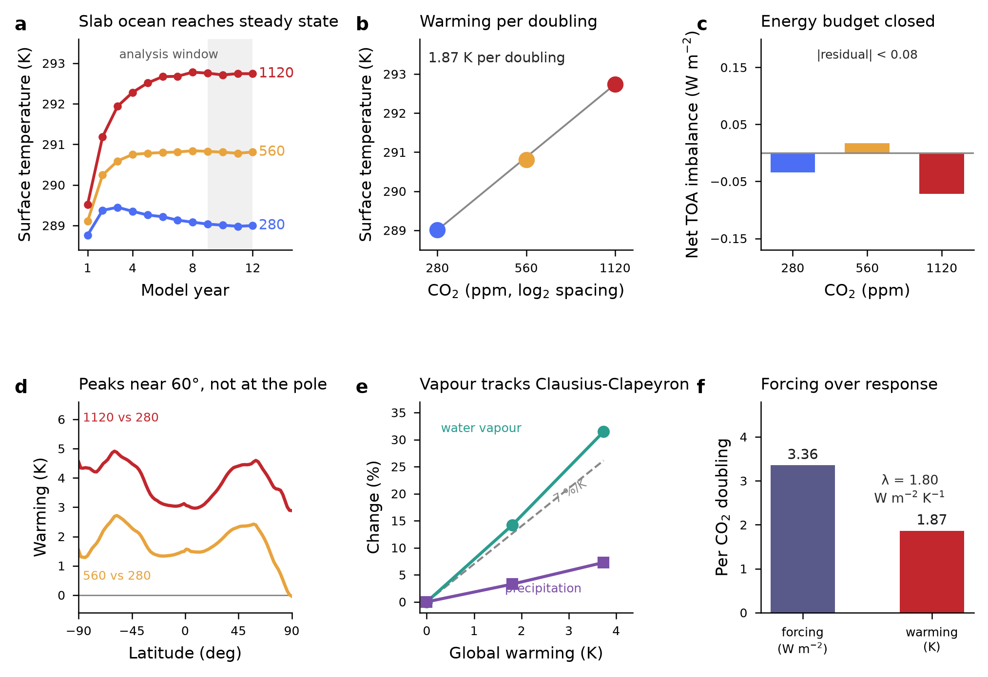
At 280, 560, and 1,120 ppm, fixed-temperature runs isolate energy forcing while slab-ocean runs allow warming. Select a saved scenario below to compare the results.
Idealized aquaplanet with a 30 m slab ocean, without realistic land, sea ice, seasons, or ocean circulation. These responses are not an Earth climate-sensitivity estimate.
Three CO₂ settings reuse one compiled model. Two cases run concurrently, then the third starts when a node becomes free.
About 24 minutes from submission to completion for the three fixed-ocean-temperature cases, including boot and queue time. The separate slab-ocean runs, setup and analysis are outside this clock.
Playback length is separate from simulated time and the session span.
Six experiments separate the added energy from the warming.
Adding CO₂ changes how the atmosphere exchanges energy. Temperature is the response, and separating the two helps explain what the model is doing. Laplace ran six CESM experiments: 280, 560, and 1,120 ppm, each with a fixed sea-surface temperature and with a 30 m slab ocean allowed to warm. Choose an experiment and concentration to inspect the saved results.
Study scope. Idealized aquaplanet with a 30 m slab ocean, without realistic land, sea ice, seasons, or ocean circulation. These responses are not an Earth climate-sensitivity estimate.
3.36 W/m²Approximate forcing increment per CO₂ doubling in this setupSource ↗
1.87 KApproximate warming per doubling in this idealized slab-ocean setupSource ↗
Explore recorded results · 6 completed model runs
Turn up the CO₂. What changes?
Choose a concentration and an experiment. The display switches between the actual saved results, with the physical assumptions kept visible.
Which question are we asking?
Temperature rise relative to 280 ppm (K)
Dots are the three saved runs. The dashed connector is a visual guide; intermediate concentrations were not simulated here.
Warming vs 280 ppm+1.80 KSlab-ocean equilibrium comparison
Mean model surface temperature17.66 °CYears 9–12 of a 12-year model run
This is an idealized aquaplanet. The slab ocean is 30 m deep; there is no realistic land, sea ice, seasons or ocean circulation. These are conditional model responses, not an Earth climate-sensitivity estimate.
How the investigation developed.
A convincing warming chart needs a controlled experiment. Changing a setup label is not enough: the actual radiation input must receive the intended CO₂ value.
01
Turn a broad request into controlled experiments
After the user specified CESM, the study compared 280, 560 and 1,120 ppm in two setups: fixed sea-surface temperature and a 30 m slab ocean.
02
Verify the setting reaches the physics
The record identified a parameter-propagation issue and checked co2vmr in the atmosphere input. Otherwise different case labels could represent the same radiative input.
03
Separate forcing from warming
Fixed-SST experiments ran 14 model months; slab-ocean experiments ran 12 model years. The selected analysis uses the final 12 months and years 9–12 respectively.
04
Deliver an interpretable comparison
Two diagnostic tables, two original figures, reduced model files, explanatory movies and a five-page report carry the experiment into a reviewable handoff.
How Laplace carried the work
Direct the investigation. Inspect the work.
Laplace carries technical execution while researchers set the question, steer the study, and evaluate the evidence.
A team-managed workflowIllustrative workflow with existing tools
Task 1Design controls
→
Task 2Configure six cases
→
Task 3Run both setups
→
Task 4Compare diagnostics
→
Task 5Write + visualize
The team coordinates tools, context, and revisions across the study.
With LaplaceTechnical work demonstrated in these studies
HUMANBrief + steer
Laplace carries the technical work
Build six casesVerify CO₂ inputCompare responsesPackage the study
↺ Run → inspect → revise, with researcher steering
HUMANReview + decide
A matrix of experiments from one briefSix configured runs replace separate manual assembly of each comparison.
Input verification inside the loopThe CO₂ setting was checked where it enters the actual atmosphere model.
Analysis + communication packagedTables, original figures, movies and a report share the same study record.
Illustrates work ownership. Box widths are schematic; human time saved was not measured.
Inspect the work inside the Laplace block
Build six cases. After the user specified CESM, the study compared 280, 560 and 1,120 ppm in two setups: fixed sea-surface temperature and a 30 m slab ocean.
Verify CO₂ input. The record identified a parameter-propagation issue and checked co2vmr in the atmosphere input. Otherwise different case labels could represent the same radiative input.
Compare responses. Fixed-SST experiments ran 14 model months; slab-ocean experiments ran 12 model years. The selected analysis uses the final 12 months and years 9–12 respectively.
Package the study. Two diagnostic tables, two original figures, reduced model files, explanatory movies and a five-page report carry the experiment into a reviewable handoff.
Original slab-ocean figure. The temperature response is conditional on this simplified world.How to read the timing
These investigations often continued across separate visits. The first and last messages do not measure continuous work.
21h 19m 49sCalendar span of the conversation
8h 14mCombined child-agent windows, with overlapping intervals counted once
Agent windows can include waiting and omit work in the main conversation. They are not a measure of active human work, total compute or time saved. The exports do not provide a reliable labour clock.
Scientific assumptions and limitations
The aquaplanet has no realistic land, sea ice, seasons or ocean circulation. Its 1.87 K response is not an estimate of Earth’s climate sensitivity.
The maximum absolute final slab-ocean energy imbalance is about 0.072 W/m²; that is a model diagnostic, not real-world validation.
A five-page article and persuasive movie do not independently establish predictive accuracy.
The record includes human direction and revisions; human effort and compute costs were not measured as a matched baseline.
The next useful decision
Repeat with richer physical components and independent validation before making an Earth-system prediction.
what is the compute power modal.com use?what is the compute power modal.com use?what is the compute power modal.com use?
Research prompt↑
LLaplaceRecorded result
A compute research note.
The conversation compares scientific-cluster and elastic-cloud hardware. It provides historical research context; no matched performance experiment was run.
No simulation or matched performance benchmark. Historical hardware and pricing claims are not current buying advice.
Infrastructure inspection makes the available CPU, memory and GPU limits explicit before a simulation is assigned to a machine.
Historical hardware inventory. The 192-core figure describes a recorded cluster node, not a workload executed or a measured speed advantage here.
A compute choice still needs a workload benchmark.
A fast chip does not automatically make a scientific program faster. Some models need many CPUs communicating efficiently; some rendering or learning tasks fit GPUs. The useful question is which resource fits the workload.
Study scope. No simulation or matched performance benchmark. Historical hardware and pricing claims are not current buying advice.
Inspect the output
This research note is preserved in the conversation; no separate artifact was supplied.
General hardware specifications are easy to mistake for a measured performance advantage on a particular model.
01
Ask what resources are available
The user asked about Modal’s compute, then narrowed the question to CPU and HPC hardware comparisons.
02
Frame the workload tradeoff
The discussion compares elastic resources with the existing cluster. It supplies a historical narrative, not a benchmark run.
03
Separate useful research from unsupported claims
Source review flagged unsupported statements about an unrelated cluster task. Those statements are excluded from the evidence used here.
How Laplace carried the work
Direct the investigation. Inspect the work.
Laplace carries technical execution while researchers set the question, steer the study, and evaluate the evidence.
A team-managed workflowIllustrative workflow with existing tools
Task 1Collect specifications
→
Task 2Map workloads
→
Task 3Compare constraints
→
Task 4Verify claims
→
Task 5Record a decision
The team coordinates tools, context, and revisions across the study.
With LaplaceTechnical work demonstrated in these studies
HUMANBrief + steer
Laplace carries the technical work
Research resourcesCompare workloadsQualify the claims
↺ Run → inspect → revise, with researcher steering
HUMANReview + decide
A decision frame gatheredCompare resource fit before choosing by headline specifications.
Research kept with the projectThe discussion remains discoverable alongside the workloads.
No invented outputThe reader preserves the source response without fabricating a chart or speed claim.
Illustrates work ownership. Box widths are schematic; human time saved was not measured.
Inspect the work inside the Laplace block
Research resources. The user asked about Modal’s compute, then narrowed the question to CPU and HPC hardware comparisons.
Compare workloads. The discussion compares elastic resources with the existing cluster. It supplies a historical narrative, not a benchmark run.
Qualify the claims. Source review flagged unsupported statements about an unrelated cluster task. Those statements are excluded from the evidence used here.
These investigations often continued across separate visits. The first and last messages do not measure continuous work.
00h 37m 51sCalendar span of the conversation
6mCombined child-agent windows, with overlapping intervals counted once
Agent windows can include waiting and omit work in the main conversation. They are not a measure of active human work, total compute or time saved. The exports do not provide a reliable labour clock.
Scientific assumptions and limitations
This is research, not a simulation. Hardware offers and prices in the historical discussion are not current recommendations.
The session does not establish that Modal is faster, cheaper or suitable for a specific MPI workload.
Review flagged unsupported claims about a separate task; the record is not proof of reliable unattended coordination.
The next useful decision
Benchmark the same approved workload and configuration on both candidate environments, including cost and transfer overhead.
Inside the first 50 milliseconds of a lunar impact.
The prompt → the result
Impact physicsRecorded session
YYouOriginal prompt
use castro to calculate asteriod collision impact with the moonuse castro to calculate asteriod collision impact with the moonuse castro to calculate asteriod collision impact with the moon
Research prompt↑
LLaplaceRecorded result
The first 50 milliseconds of impact.
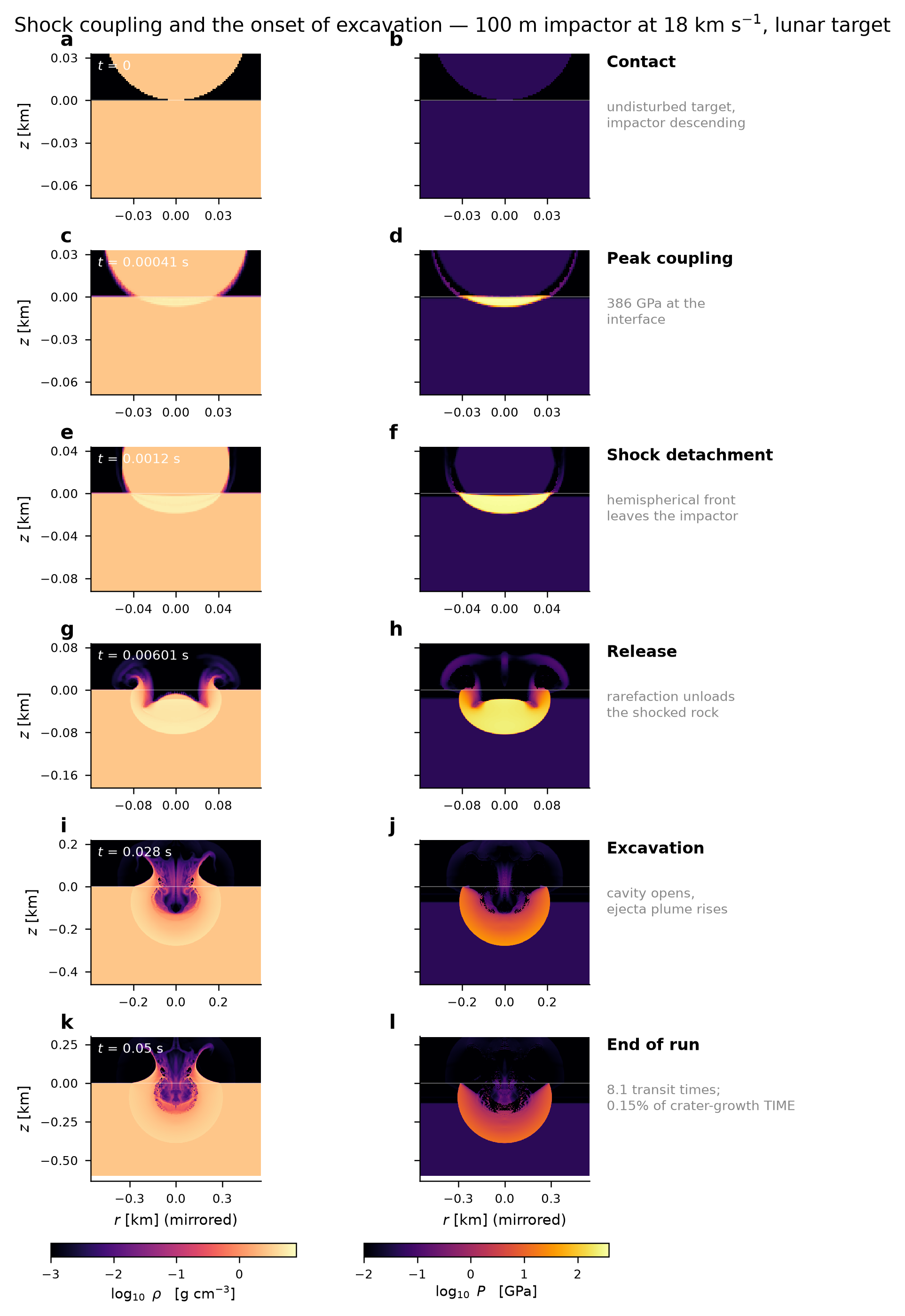
The lunar-impact chapter recorded a peak pressure of about 385.7 GPa, compared with a 391.4 GPa analytic reference. Earlier chapters explored fluid instability and a stellar-layer toy.
The impact simulation ends at 0.05 seconds. The final-crater estimate comes from a separate scaling law; the stellar example is an idealized toy.
This request steered an ongoing investigation. The result summarizes the recorded session, including later requests and review. The opening pairs the lunar-impact request with its chapter; fluid and stellar chapters follow below.
Read the research prompt
Original research prompt
use castro to calculate asteriod collision impact with the moon
Adaptive refinement concentrates resolution around the shock while parallel processors advance the impact model and record its evolution.
Recorded runtime for the final early-impact run, covering 0.05 physical seconds. Preparation, physics corrections, validation and movies are outside this clock.
Playback length is separate from simulated time and the session span.
One solver investigation reaches from falling fluid to a lunar impact.
What happens in the first instant after a rock strikes the Moon? This session built a Castro investigation spanning fluid instability, a stellar-layer toy, and a short lunar-impact calculation. The impact chapter resolves the early shock and compares a peak pressure with an analytic reference. Final crater formation lies beyond the simulated window.
Study scope. The impact simulation ends at 0.05 seconds. The final-crater estimate comes from a separate scaling law; the stellar example is an idealized toy.
Original early-impact snapshots. The evolving cavity is not a final crater.
How the investigation developed.
Starting from a new solver requires environment knowledge, problem setup, numerical debugging, diagnostics and communication.
01
Chapter 1 · create a specialist and test an instability
The session starts with a Castro specialist, then demonstrates Rayleigh–Taylor instability in 2D and 3D: heavy fluid falling through lighter fluid.
02
Chapter 2 · explore a stellar-layer toy
An imposed heat pulse drives motion in a two-dimensional plane-parallel atmosphere. The output measures material leaving the computational top boundary. It is not a magnetized solar-ejection model.
03
Chapter 3 · simulate a lunar impact’s early shock
A 100 m rock strikes at 18 km/s in a 2D axisymmetric setup with a custom equation of state. The calculation covers only the first 0.05 seconds.
04
Compare and qualify the output
The recorded impact peak pressure is about 385.7 GPa versus a 391.4 GPa analytic reference. A 2.21 km final crater estimate comes from a scaling law, not the short simulation.
How Laplace carried the work
Direct the investigation. Inspect the work.
Laplace carries technical execution while researchers set the question, steer the study, and evaluate the evidence.
A team-managed workflowIllustrative workflow with existing tools
Task 1Learn Castro
→
Task 2Configure problems
→
Task 3Run + debug
→
Task 4Audit diagnostics
→
Task 5Write reports
The team coordinates tools, context, and revisions across the study.
With LaplaceTechnical work demonstrated in these studies
HUMANBrief + steer
Laplace carries the technical work
Build + test CastroRun stellar toyRun impact studyCompare + qualify
↺ Run → inspect → revise, with researcher steering
HUMANReview + decide
A solver setup reused within a sessionThe record moves from capability setup into several explicit study requests.
Diagnostics carried into reportsImages, numerical metrics and two papers accompany the demonstrations.
Model boundaries made explicitEarly shock, domain mass loss and scaling estimates remain separate claims.
Illustrates work ownership. Box widths are schematic; human time saved was not measured.
Inspect the work inside the Laplace block
Build + test Castro. The session starts with a Castro specialist, then demonstrates Rayleigh–Taylor instability in 2D and 3D: heavy fluid falling through lighter fluid.
Run stellar toy. An imposed heat pulse drives motion in a two-dimensional plane-parallel atmosphere. The output measures material leaving the computational top boundary. It is not a magnetized solar-ejection model.
Run impact study. A 100 m rock strikes at 18 km/s in a 2D axisymmetric setup with a custom equation of state. The calculation covers only the first 0.05 seconds.
Compare + qualify. The recorded impact peak pressure is about 385.7 GPa versus a 391.4 GPa analytic reference. A 2.21 km final crater estimate comes from a scaling law, not the short simulation.
Original figure. About 1.76% mass leaving the open top is domain loss, not evidence that material escaped the Sun.How to read the timing
These investigations often continued across separate visits. The first and last messages do not measure continuous work.
1d 00h 05m 55sCalendar span of the conversation
6h 20mCombined child-agent windows, with overlapping intervals counted once
Agent windows can include waiting and omit work in the main conversation. They are not a measure of active human work, total compute or time saved. The exports do not provide a reliable labour clock.
Scientific assumptions and limitations
These are three chapters in one session, not three independent customer successes.
The stellar toy omits magnetic fields and does not model a solar coronal mass ejection.
The impact calculation ends before final crater formation; the 2.21 km estimate is a separate scaling-law result.
Equation-of-state, diagnostic, literature and audit issues were revised during the record. The supplied reports are not an independent validation or a fully reconciled reproducibility package.
Melt thresholds and mass estimates involve additional assumptions; the reader does not promote them as verified physical predictions.
The next useful decision
Reconcile the final input and diagnostic package, then validate the intended regime against an independent benchmark before extending the model.
Different underground models. Similar magnetic signals.
The prompt → the result
Magnetic geophysicsRecorded session
YYouOriginal prompt
create a 3D simulation of that; with real earth datacreate a 3D simulation of that; with real earth datacreate a 3D simulation of that; with real earth data
Research prompt↑
LLaplaceRecorded result
Two underground models fit the signal.
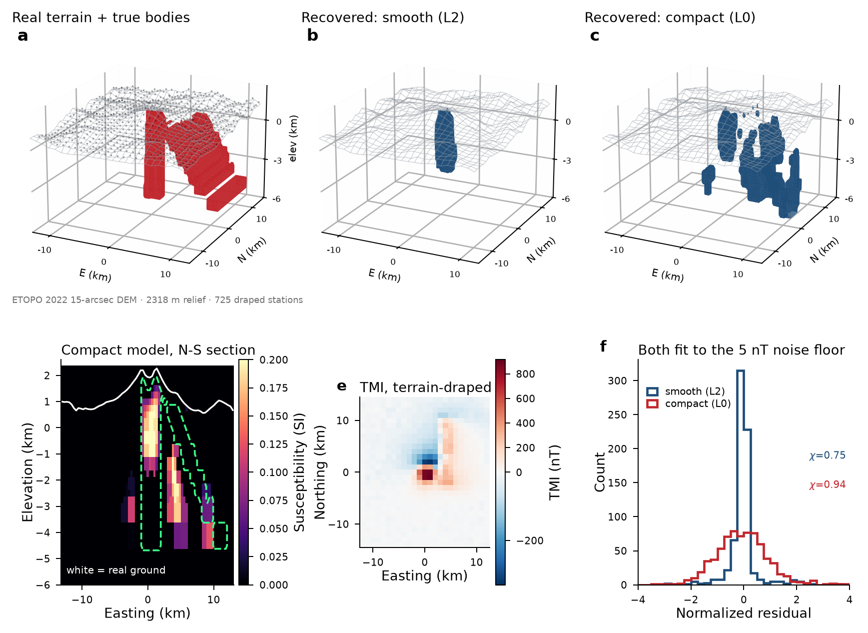
A 725-station synthetic magnetic survey over real terrain supported different recovered models. The comparison made non-uniqueness visible.
Synthetic magnetic observations and buried structures over real terrain. Fit ratios are not reconstruction-accuracy percentages.
A terrain-aware model creates 725 synthetic observations, then solves the same inverse problem with both smooth and compact assumptions.
Recorded computation over real Mount St Helens terrain, with synthetic magnetic observations. The 108 seconds excludes research iterations and animation; different subsurface models can fit the same data.
Watch the result Original session films
Inspect the 3D reconstruction6s playback
A rotating view of the Mount St Helens experiment: real terrain, 725 synthetic survey stations, and smooth versus compact reconstructions. The underground structures and magnetic observations are constructed, not field measurements.
Why fitting the signal is not enough1m 6.5s playback
A Manim explainer from the earlier 441-station synthetic experiment in this session. It combines schematic geometry with recorded SimPEG results to explain why different underground models can fit the signal. This is a different example from the 725-station terrain study.
Playback length is separate from simulated time and the session span.
108,484 cells. Two plausible underground reconstructions.
Inferring underground rock from a magnetic signal is like guessing an object from its shadow. More than one shape can fit. This study makes that ambiguity visible by reconstructing the same synthetic survey with two different preferences for underground structure.
Study scope. Synthetic magnetic observations and buried structures over real terrain. Fit ratios are not reconstruction-accuracy percentages.
725 stationsSynthetic magnetic survey locations over real terrainSource ↗
Original figure compares the known constructed bodies with smooth and compact reconstructions. It is not a discovery beneath Mount St Helens.
How the investigation developed.
A visually convincing underground reconstruction can hide a dependence on modelling assumptions and regularization.
01
Build and test the SimPEG capability
Laplace built a SimPEG workflow, starting with numerical checks and synthetic magnetic examples before moving to a three-dimensional terrain model.
02
Place an experiment on real terrain
The Mount St Helens example uses NOAA ETOPO terrain and a specified IGRF field, but its subsurface bodies and magnetic anomaly are synthetic.
03
Compare two valid-looking answers
A smooth and a compact inversion both fit the constructed signal while distributing susceptibility differently underground.
04
Explain non-uniqueness
Original figures and movies visualize what changes between the models. Review corrected a misfit-target definition and an earlier illustrative animation trace.
How Laplace carried the work
Direct the investigation. Inspect the work.
Laplace carries technical execution while researchers set the question, steer the study, and evaluate the evidence.
A team-managed workflowIllustrative workflow with existing tools
Task 1Acquire terrain
→
Task 2Construct a survey
→
Task 3Configure inversions
→
Task 4Compare models
→
Task 5Explain ambiguity
The team coordinates tools, context, and revisions across the study.
With LaplaceTechnical work demonstrated in these studies
HUMANBrief + steer
Laplace carries the technical work
Test SimPEGBuild terrain modelCompare inversionsExplain uncertainty
↺ Run → inspect → revise, with researcher steering
HUMANReview + decide
Multiple models compared in one workflowTwo inversion choices expose what a single polished reconstruction would conceal.
Data + geometry assembledReal topography is brought into a controlled synthetic experiment.
A decision-ready uncertainty storyThe explanation makes the need for another measurement concrete.
Illustrates work ownership. Box widths are schematic; human time saved was not measured.
Inspect the work inside the Laplace block
Test SimPEG. Laplace built a SimPEG workflow, starting with numerical checks and synthetic magnetic examples before moving to a three-dimensional terrain model.
Build terrain model. The Mount St Helens example uses NOAA ETOPO terrain and a specified IGRF field, but its subsurface bodies and magnetic anomaly are synthetic.
Compare inversions. A smooth and a compact inversion both fit the constructed signal while distributing susceptibility differently underground.
Explain uncertainty. Original figures and movies visualize what changes between the models. Review corrected a misfit-target definition and an earlier illustrative animation trace.
These investigations often continued across separate visits. The first and last messages do not measure continuous work.
08h 52m 41sCalendar span of the conversation
32mCombined child-agent windows, with overlapping intervals counted once
Agent windows can include waiting and omit work in the main conversation. They are not a measure of active human work, total compute or time saved. The exports do not provide a reliable labour clock.
Scientific assumptions and limitations
Terrain is real; the magnetic observations and buried structures are synthetic.
The reconstruction depends on the specified field, geometry and inversion assumptions.
Misfit ratios measure fit relative to an assumed noise model, not the probability that the geology is correct.
The supplied archive is a partial set of the artifact records.
The next useful decision
Add an independent subsurface constraint or a differently sensitive survey to distinguish the competing models.
A good gravity fit can still leave depth uncertain.
The prompt → the result
Gravity geophysicsRecorded session
YYouOriginal prompt
use SemPeg, think about some kind of data you get from your earthdata API, and apply a 3D simulation by SImPeg trying to understand and explain the datause SemPeg, think about some kind of data you get from your earthdata API, and apply a 3D simulation by SImPeg trying to understand and explain the datause SemPeg, think about some kind of data you get from your earthdata API, and apply a 3D simulation by SImPeg trying to understand and explain the data
Research prompt↑
LLaplaceRecorded result
A close data fit, with depth still unresolved.
When real-data acquisition failed, the study used a synthetic gravity example. A near-target misfit and mass recovery did not establish reliable depth recovery.
Synthetic substitute after real-data acquisition failed. The original figure retains a misleading BedMachine label; depth recovery remains unresolved.
The result summarizes the recorded session, including later requests and review.
Read the research prompt
Original research prompt
use SemPeg, think about some kind of data you get from your earthdata API, and apply a 3D simulation by SImPeg trying to understand and explain the data
An integral formulation avoids unavailable sparse solvers; parameter searches test the reconstruction against known synthetic geometry.
A synthetic stand-in after real-data access failed. Eight iterations describes the accepted fit, not elapsed time. The recovered model still does not resolve absolute bed depth.
Watch the result Original session films
The fit and its blind spot1m 8.1s playback
Original explanation of a synthetic gravity inversion.
Playback length is separate from simulated time and the session span.
529 synthetic observations expose the limits of a good gravity fit.
Gravity measurements contain clues about material below the surface, but several underground arrangements can produce similar readings. A model can match those readings and still put material at the wrong depth. This case makes that limitation visible.
Study scope. Synthetic substitute after real-data acquisition failed. The original figure retains a misleading BedMachine label; depth recovery remains unresolved.
529 stationsSynthetic observations used in the inverse problemSource ↗
1.012Final data-misfit ratio, not reconstruction accuracySource ↗
+5.02%Recovered mass relative to constructed truthSource ↗
Original figure retained unchanged. Its “BedMachine geometry” legend refers to the synthetic stand-in used in this run, not a downloaded real bed dataset.
How the investigation developed.
The user wanted real Earth data. Access to BedMachine was blocked, so the recorded study substituted synthetic geometry. That change determines what the result can claim.
01
Disclose the data substitution
The study uses a synthetic stand-in, not the requested real BedMachine dataset. The source report records the access problem.
02
Build and invert a gravity experiment
The model uses 49,376 active cells and 529 synthetic stations. Review corrected a thousand-fold unit issue and rejected an optimizer exit code as sufficient convergence evidence.
03
Check the answer against known synthetic truth
The recovered mass is about 5.02% above the constructed truth, and the along-axis position is close, but the bed-depth geometry remains unresolved.
04
Deliver both fit and failure
The report, scorecard, figures and movie show why a near-target data misfit is insufficient for a trustworthy depth estimate.
How Laplace carried the work
Direct the investigation. Inspect the work.
Laplace carries technical execution while researchers set the question, steer the study, and evaluate the evidence.
A team-managed workflowIllustrative workflow with existing tools
Task 1Acquire data
→
Task 2Build gravity model
→
Task 3Invert observations
→
Task 4Check geometry
→
Task 5Prepare a handoff
The team coordinates tools, context, and revisions across the study.
With LaplaceTechnical work demonstrated in these studies
HUMANBrief + steer
Laplace carries the technical work
Disclose stand-inRun gravity inversionCheck known truthExplain depth limits
↺ Run → inspect → revise, with researcher steering
HUMANReview + decide
Troubleshooting connected to interpretationUnit, optimizer and regularization issues are recorded with their scientific consequences.
Failure becomes useful evidenceThe comparison exposes unresolved depth even when the data fit looks good.
Reusable diagnostic handoffA scorecard, sections, report and movie preserve the result and its limits.
Illustrates work ownership. Box widths are schematic; human time saved was not measured.
Inspect the work inside the Laplace block
Disclose stand-in. The study uses a synthetic stand-in, not the requested real BedMachine dataset. The source report records the access problem.
Run gravity inversion. The model uses 49,376 active cells and 529 synthetic stations. Review corrected a thousand-fold unit issue and rejected an optimizer exit code as sufficient convergence evidence.
Check known truth. The recovered mass is about 5.02% above the constructed truth, and the along-axis position is close, but the bed-depth geometry remains unresolved.
Explain depth limits. The report, scorecard, figures and movie show why a near-target data misfit is insufficient for a trustworthy depth estimate.
These investigations often continued across separate visits. The first and last messages do not measure continuous work.
01h 40m 19sCalendar span of the conversation
25mCombined child-agent windows, with overlapping intervals counted once
Agent windows can include waiting and omit work in the main conversation. They are not a measure of active human work, total compute or time saved. The exports do not provide a reliable labour clock.
Scientific assumptions and limitations
The requested real-data acquisition did not succeed; the demonstrated study is synthetic.
Matching the data does not establish bed-depth recovery. Residual bias also remains in the scorecard.
Mass and position errors concern this chosen synthetic truth and noise model, not field performance.
The original figure retains a misleading BedMachine label, explicitly qualified here.
The next useful decision
Obtain the intended dataset, then add independent depth information and repeat the inversion with an appropriate uncertainty analysis.
use openfoam to do a RANS turbulence modeling of supersonic gas eductoruse openfoam to do a RANS turbulence modeling of supersonic gas eductoruse openfoam to do a RANS turbulence modeling of supersonic gas eductor
Research prompt↑
LLaplaceRecorded result
A diagnosis, with performance unresolved.
The staged CFD case reached 410,400 cells, but mass imbalance remained around 50%. The useful output was the failure diagnosis and a proposed next solver test.
No accepted entrainment ratio. A transient-solver alternative was proposed but not run successfully in this record.
A large flow model is paired with automated checks that reveal mass imbalance and wall-treatment failures before a design claim is accepted.
The case remains unconverged. Rank counts describe attempted runs; no accepted entrainment result or measured speedup was produced.
A failed coarse run challenges the case for a much larger mesh.
An eductor uses a high-speed gas stream to pull in another stream. Engineers care how much it entrains. This session shows why a solver that runs for longer is not enough: the flow must also converge and conserve mass before its performance number is useful.
Study scope. No accepted entrainment ratio. A transient-solver alternative was proposed but not run successfully in this record.
Original diagnostic figure. Grouped early-failure bars are representative; exact early iteration counts vary. Longer survival does not establish convergence.
How the investigation developed.
A difficult compressible-flow setup can tempt a team to invest in larger meshes before isolating the actual failure.
01
Build the OpenFOAM setup
The record develops a specialist and a steady compressible RANS case with a k–ω SST turbulence model.
02
Challenge the mesh explanation
A 51,300-cell coarse case also fails, weakening the claim that fine-grid geometry alone explains the problem. The proposed very large remesh was not executed.
03
Improve numerical survival without accepting the answer
After revised turbulence initialization, one reported run reaches about 1,150 iterations but still fails. Residuals and mass balance remain unacceptable.
04
Preserve the diagnosis and next proposal
The final staged case has 410,400 cells. A transient solver and inlet-boundary revision are proposed next, not demonstrated as successful.
How Laplace carried the work
Direct the investigation. Inspect the work.
Laplace carries technical execution while researchers set the question, steer the study, and evaluate the evidence.
A team-managed workflowIllustrative workflow with existing tools
Task 1Define the flow
→
Task 2Mesh the geometry
→
Task 3Configure solver
→
Task 4Diagnose instability
→
Task 5Plan the next test
The team coordinates tools, context, and revisions across the study.
With LaplaceTechnical work demonstrated in these studies
HUMANBrief + steer
Laplace carries the technical work
Build flow caseTest mesh hypothesisDiagnose failed runPropose bounded test
↺ Run → inspect → revise, with researcher steering
HUMANReview + decide
An expensive branch challengedA failed coarse run weakened the case for the proposed large remesh.
False success rejectedIteration count and optimizer survival are separated from physical convergence.
A bounded next experimentThe handoff identifies an unresolved result and a specific next test.
Illustrates work ownership. Box widths are schematic; human time saved was not measured.
Inspect the work inside the Laplace block
Build flow case. The record develops a specialist and a steady compressible RANS case with a k–ω SST turbulence model.
Test mesh hypothesis. A 51,300-cell coarse case also fails, weakening the claim that fine-grid geometry alone explains the problem. The proposed very large remesh was not executed.
Diagnose failed run. After revised turbulence initialization, one reported run reaches about 1,150 iterations but still fails. Residuals and mass balance remain unacceptable.
Propose bounded test. The final staged case has 410,400 cells. A transient solver and inlet-boundary revision are proposed next, not demonstrated as successful.
These investigations often continued across separate visits. The first and last messages do not measure continuous work.
14h 25m 04sCalendar span of the conversation
53mCombined child-agent windows, with overlapping intervals counted once
Agent windows can include waiting and omit work in the main conversation. They are not a measure of active human work, total compute or time saved. The exports do not provide a reliable labour clock.
Scientific assumptions and limitations
The conversation is marked completed, but the CFD investigation is unresolved. No entrainment ratio is accepted.
The source report contains earlier hypotheses alongside later addenda; the later diagnostic evidence weakens the initial mesh-only explanation.
The transient-solver alternative is a proposal, not an executed successful follow-on.
Source review raised compute-authorization issues. This record is not proof of unattended spend control.
The next useful decision
Review the boundary conditions, then authorize and validate a bounded transient test with explicit convergence and mass-balance acceptance criteria.
Each study connects its physical question to the recorded result, model assumptions and selected scientific files.
Numerical results with their limits
Synthetic observations, reduced models and comparisons between solvers are identified in the study. Numerical agreement does not by itself establish physical validation.
A focused technical handoff
Explore selected tables, figures, movies and scientific Python scripts. The public evidence summaries are curated explanations. Some original inputs and dependencies are unavailable, so the downloads are not complete reproducibility packages.